New in Microsoft Excel 2019 (Standard or 365)

Excel 2019 has a few new features coming, including some new handy functions which will probably be the newcomers that you are most likely to use. We’ll write up more about these new features once we have experience of using them in practice.

A couple of big points to note now though are:

• If you have Microsoft 365 (what was called Office 365) then you will probably already have the new Excel functions for 2019 now.
• Excel 2019 is not compatible with Windows 7 or 8 or 8.1. It is compatible only with Windows 10 onwards (or Mac).
• If you have Microsoft 365/Office 365 but you are using an earlier version than Windows 10, then you won’t have all of the new Excel 2019 features.
• As always, if you want to share a spreadsheet with users who are not on Excel 2019 (or 365) then do not use the new functions. You need to make sure that your file only uses functions that are compatible with the earliest version of Excel that the people who open your file have.

In the meantime, the full list of new functions currently available only in Excel 365 or Excel 2019 is: CONCAT, IFS, MINIFS, MAXIFS, SWITCH, TEXTJOIN and some specialist FORECAST functions. Here are some examples of how these can be used in practice:

These functions are for stringing together pieces of text across a range of cells. It's easier to see this in practice in our download file, but here is some explanation too:

So, suppose you had first names, middle names and surnames of people arranged across 3 columns, you could CONCAT these together to spell out the full names of the people. The only snag here is that there are no spaces between the names, so you would need to insert columns in between containing just a space for it to work.

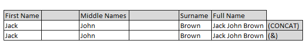
The advantage of this method of joining pieces of text is that you don't have to identify each cell you want included individually. Instead you select the range, for example =CONCAT(K14:O14).

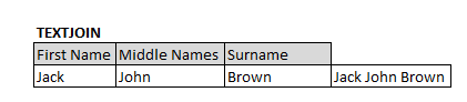
A better choice in this situation, however, would be the TEXTJOIN function, which allows you to specify a separator and allows you to ignore empty cells so that you don't end up with extra separators

e.g. =TEXTJOIN(" ", TRUE, A16:C16)

Another example of where TEXTJOIN is useful is when building a list of items from separate cells, where you can use "," as your separator.

Alternative ways of stringing text together (also known as concatenating) are:

- use the & (ampersand) operator: = K14 & L14 & M14 & N14 & O14.

Here you have to specify individual cells, but you can insert your own variations so you could create the name as surname, first name middle names. This might look like

= O14 & ", " & K14 & " " & M14

- use the CONCATENATE function: = CONCATENATE(K14, L14, M14, N14, O14)

This offers no advantages over the & method, but you can still be more flexible with the order and in between bits

= CONCATENATE(O14, ", ", K14, " ", M14)

You can see all of these functions in action in our download file.

This function allows you to specify multiple criteria and results without having to use nested IF functions. This makes a formula much easier to read, understand and edit than if you use nested IF functions.

This is best seen by example in our download file, in cells C5 and B5.

But here's an explanation in words:

Suppose you want to be able to enter a date and find out whether it is a weekend, a public holiday, part of the summer shutdown period or just a normal working day.

You would set up a list of public holiday dates, which you name as a range "HolidaysList"

And you could designate a cell where you enter your data and name that "MyDate".

Using nested IF functions, you might enter a formula like this:

=IF(OR(WEEKDAY(MyDate)=6,WEEKDAY(MyDate)=7), "Weekend", IF(ISNUMBER(MATCH(MyDate, HolidaysList, 0)), "Public Holiday", IF(MONTH(MyDate)=7, "Summer shutdown", "Working day")))

Broken down into English, this says :

If MyDate is a Saturday or a Sunday the answer is "Weekend",

Otherwise if there's a match for my date in the HolidaysList the answer is "Public Holiday"

Otherwise if the month of MyDate is July the answer is "Summer shutdown"

Otherwise it's a "Working day"

Presenting this via the new IFS function looks like this:

=IFS(OR(WEEKDAY(MyDate)=6, WEEKDAY(MyDate)=7), "Weekend", ISNUMBER(MATCH(MyDate, HolidaysList, 0)), "Public Holiday", MONTH(MyDate)=7, "Summer shutdown", TRUE, "Working day")

This reads off in English in exactly the same way, but doing it this way, you don't need to keep starting another IF function so that it's easier to do the reading of the pairs of criteria checks with answers.

Note though, the extra "TRUE" inserted nearly at the end so that you can specify what the answer is if all else fails.

These functions best apply to database-type data. Here, typically, you have column headings for various attributes and then each row represents a record of data about something. You can see data set out like this in our download file, on the MinIfs MaxIfs sheet.

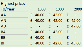
In our example, we have details of sale prices for various reps per year to our customers.

The MINIFS function enables you to look through data to find the minimum value of something, subject to multiple criteria. So, in our example we have found the minimum price sold at for each rep and year. You can see this in the pink table.

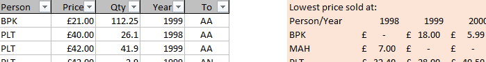
The formula looks something like:

=MINIFS(PriceColumn, RepColumn, MyRep, YearColumn, MyYear)

where each of those words will be replaced by a cell or range of cells. E.g. PriceColumn will be the whole column of prices.

And reading this in English, we say

Find the minimum value in the price column

where the rep column value is the rep I am interested in

and the year column value is the year I am interested in.

The MAXIFs function works in exactly the same way but enables you to find the maximum value instead. You can see this in the green table in our example, where we have shown the figures per customer sold to.

The formula looks something like:

=MAXIFS(PriceColumn, ToColumn, MyCustomer, YearColumn, MyYear)

where each of those words will be replaced by a cell or range of cells. E.g. ToColumn will be the whole column of customers sold to.

Find the maximum value in the price column

where the To column value is the customer I am interested in

and the year column value is the year I am interested in.

The pink and green examples could actually be achieved using a pivot table, rather than functions.

These are shown in the blue areas, for information only. Pivot tables have the advantage that they automatically create the lists of reps or customers for you. On the other hand, they do not update automatically if your data changes as you have to manually refresh them. The MINIFS and MAXIFS functions - like all functions - do update automatically under normal circumstances.

We have created a further example, in yellow in the download file, which applies an extra criterion and so cannot so easily be created using a pivot table.

Here, the formula looks something like:

=MINIFS(PriceColumn, RepColumn, MyRep, YearColumn, MyYear, QuantityColumn, ">50")

And reading this in English, we say

Find the minimum value in the price column

where the rep column value is the rep I am interested in

and the year column value is the year I am interested in

and the quantity sold is more than 50.

In Microsoft's own words, the SWITCH function evaluates one value against a list of values, and returns the result corresponding to the first matching value. If there is no match, an optional default value may be returned.

You would most likely have used a VLOOKUP function for this previously. There are pros and cons of each so here is an explanation of SWITCH and a comparison of using both.

In our download file we have an example which tests a date cell and returns either the name of that date, e.g. Christmas day, or "Not a bank holiday".

We have previously set up a list of the bank holidays in a year, and given each of them their names.

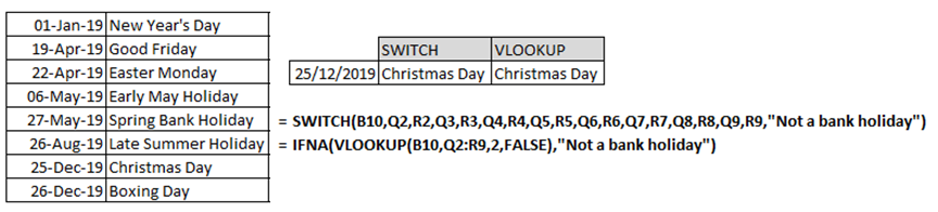
The SWITCH function looks something like:

=SWITCH(MyDate, PossibleMatch1, Name1, PossibleMatch2, Name2, PossibleMatch3, Name3, PossibleMatch4, Name4, PossibleMatch5, Name5, PossibleMatch6, Name6, PossibleMatch7, Name7, PossibleMatch8, Name8, "Not a bank holiday")

If you have a long list of possible matches, this can be tedious and prone to error to set up, especially compared to VLOOKUP.

But note the last part of the formula, where you can specify what to do if there is no match. VLOOKUP does not provide this option on its own and always returns "#NA" in that situation.

The equivalent, using VLOOKUP, looks something like:

=IFNA(VLOOKUP(MyDate, DatesAndNamesList, 2, FALSE), "Not a bank holiday")

Note that we have used the IFNA function to specify that if the VLOOKUP does not find a match and so returns #NA, it should instead show "Not a bank holiday" like the SWITCH version does.

And instead of having to spell out each possible match and result, we have been able simply to find a match in the list of dates and names and return the corresponding name from the 2nd column.

So whilst SWITCH is easier to understand, once you understand VLOOKUP that is much easier to set up in practice.

Watch this space for updates as Excel 2019 becomes more widely-used. There is a detailed write-up of other new features that came along in Excel 2016 on that Excel 2016 page.

Software-Matters have been experts in bespoke Excel systems since 1995.

Find out more about how we can help you with your project by emailing us via our Contact page or giving us a call on 01747 822616. We give free advice!

If you would like to read more about the different Excel versions follow the links below.

• What's new in Microsoft Excel 2016
• What's new in Microsoft Excel 2013
• What's new in Microsoft Excel 2010
• What's new in Microsoft Excel 2007
• Benefits of using Microsoft Excel

If you enjoyed this page or found it useful, why not tell others about it?